Site menu:

cNORM - Model Validation
From a mathematical point of view, the regression function represents a so-called hyperplane in three-dimensional space. If R2 is sufficiently high (e.g. R2 > .99), this plane usually models the manifest data over wide ranges of the standardization sample very well. However, a Taylor polynomial, as used here, usually has a finite radius of convergence. This means that there are age or performance ranges for which the regression function no longer provides plausible values. With high R2, these limits of model validity are only reached at the outer edges of the age or performance range of the standardization sample or even beyond. Please note that such model limits occur not only because the method is not omnipotent, but also because the underlying test scales have only a limited validity range within which they can reliably map a latent ability to a meaningful numerical test score. In other words, the limits of model validity often show up at those points where the test has too strong floor or ceiling effects or where the standardization sample is too diluted.
Of course, norm tables and normal scores should generally only be issued within the validity range of the model and the test. It is therefore essential to determine the limits of model validity when applying cNORM (or any other procedure used to model normal scores). For this purpose, cNORM mainly provides graphical methods, which we present to you on this page. At this point, however, we would like to point out to the mathematically experienced users that it is also possible to approach the topic analytically. Since the regression equation is a polynomial of the nth degree that is very easy to handle from a mathematical point of view, it can be subjected to a conventional curve sketching. This makes it very easy to determine, for example, where extremes, turning points, saddle points, etc. occur or where the gradient has implausible values.
Below you will find three functions for checking the model fit graphically and making the limits of the model visible:
Plot Percentiles
The following figure shows how well the model generally fits the manifest data:
# Plots the fitted and the manifest percentiles
plot(model, "percentiles")
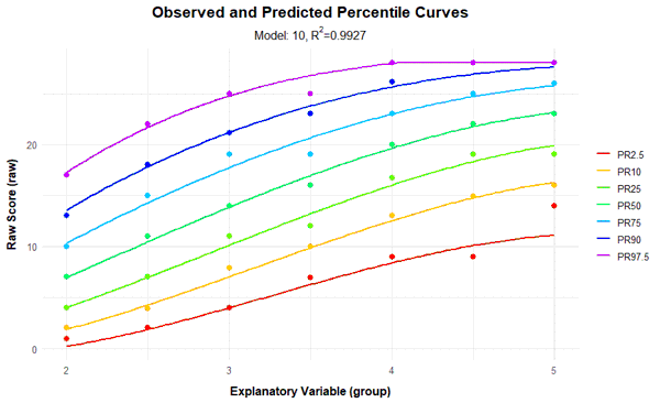
In the figure, the range of raw scores was automatically determined by the values in the original dataset, but it can be manually specified by 'minRaw = 0' and 'maxRaw = 28' (range of scores in this particular test) as well. As the figure shows, the predicted percentiles run smoothly across all levels of the explanatory variable and are in good agreement with the original data. Small fluctuations between the individual groups are eliminated. It is important to ensure that the percentile lines do not intersect, since this would mean that different values of the latent person variable are assigned to one single raw score. The mapping of latent person variables to raw scores would no longer be biunique (=bijective) at this point, e.g. it would not be possible to distinguish between these different values of the latent variable by means of the test score. As already described above, intersecting percentiles predominantly occur when the regression model is extended to age or performance ranges that do not or only rarely occur in the standardization sample, or when the test shows strong floor or ceiling effects.
If you are not sure yet, which model to choose, you can display a series of plots with an increasing number of predictors, for example:
# Displays a series of plots of the fitted and the manifest percentiles
plot(model, "series")
A drawback of the Taylor polynomials is a model misspecification in the form of intersecting percentile curves. These can be checked with the 'checkConsistency' function. Please not that extending the check to extreme values will at some point most likely find inconsictencies in the model. Here, wie restrict it to the T score range of 25 to 75:
# Search for intersecting percentiles
checkConsistency(model, minNorm = 25, maxNorm = 75)
Plot Fit of Raw Scores
In the next figure, the fitted and the manifest data are compared separately for each (age) group. Please leave 'group' empty to plot all values irrespective of group:
plot(model, "raw", group=TRUE)
The adjustment is particularly good if all points are as close as possible to the bisecting line. However, it must be noted that deviations in the extremely upper, but particularly in the extremely lower performance range often occur because the manifest data in these areas are also associated with low reliability.
Plot Fit of Norm Scores
The function plots the manifest against the fitted norm scores instead. Please also specify the limits of the norm score range, in the concrete example these are T-scores from 25 to 75. The scores thus cover the range from -2.5 to +2.5 standard deviations around the population mean.
plot(normData, "norm", group=TRUE)


Plot Density
The function plots the probability density function of the raw scores based on the regression model. Like the derivative plot function, this method can be used to identify violations of model validity or to better visualize deviations of the test results from the normal distribution.
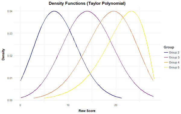
plot(model, "density", group = c (2, 3, 4))
Derivative Plot
To check whether the mapping between latent person variables and test scores is biunique, the regression function can be searched numerically within each group for bijectivity violations using the 'checkConsistency' function. In addition, it is also possible to plot the first partial derivative of the regression function to l and search for negative values. This can be done in the following way:
plot(model, "derivative")
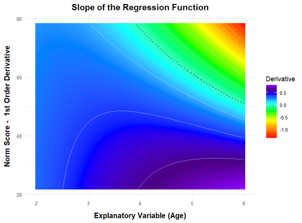
In this figure, we have extended both the age and the performance range beyond the limits of the standardization sample in order to better represent and check the limits of the model validity. (Please remember that the age variable in this norming sample comprises the values 2 to 5 and that 200 children per age group were examined.) As you can see, the first partial derivative of the regression function to l is only negative in the upper age and performance range. This does not mean that the modeling has failed, but that the test scale loses its ability to differentiate in this measuring range.
When, at the end of the modeling process, norm tables are generated, the identified limits of model validity must be respected. Or to put it in other words: Normal scores should only be issued for the valid ranges of the model.
 |
Modeling |
Norm Tables |
 |