Site menu:

cNORM - Data Preparation
Content
- Representativeness of the data base
- Weighting to compensate for violations of represantativeness
- Determining the norm sample size
- Data preparation in R
- Ranking: Retrieving Percentiles and Norm Scores
- Computing powers and interactions
- In a single step
Representativeness of the data base
The starting point for standardization should always be a representative sample. Establishing representativeness is one of the most difficult tasks of test construction and must therefore be carried out with appropriate care. First of all, it is important to identify those variables that systematically covary with the variable to be measured. In the case of school performance and intelligence tests, these are, for example, the type of school, the federal state, the socio-economic background, etc. Caution: Increasing the sample size is only beneficial for the quality of the standardization if the covariates do not remain systematically distorted. For example, it would be useless or even counterproductive to increase the size of the sample if the sample was only collected from a single type of school or only in a single region.
Weighting
If representativeness cannot be achieved and manual stratification is also difficult, the data can be weighted by means of Iterative Proportional Fitting (Raking). We have conducted extensive simulation studies (publication in preparation), which show that weighting almost always leads to better, more representative norms and usually does no harm.
Determining the norm sample size
The appropriate sample size cannot be quantified in a definitive way, but depends on how well the test (or scale) must differentiate in the extreme sections of the norm scale. In many countries, for example, it is common (although not always reasonable) to differentiate between IQ < 70 and IQ > 70 to diagnose developmental disabilities and to choose the appropriate school type or track. An IQ test used for school placement must therefore be able to identify a deviation of 2 SD or more from the population mean as reliably as possible. If, on the other hand, the diagnosis of a reading/spelling disorder is required, a deviation of 1.5 SD from the population mean is generally sufficient for the diagnosis according to DSM5. As a rule of thumb for determining the ideal sample size, it can be stated that the uncertainty of standardization increases particularly in those performance ranges which are rarely represented in the standardization sample. (This does not only apply to the nonparametric method presented here, but in principle also to all parametric standardization methods.) For example, in a representative random sample of N = 100, the probability that there is no single child with an IQ below 70 is about 10%. For a sample size of N = 200, this probability decreases to 1 %. Doubling the sample size thus notably improves the reliability of the normal score in ranges markedly deviating from the scale mean.
Since cNORM always uses the entire sample, the statistical power of the norm fitting increases. As a consequence, the norm samples can be reduced significantly. With a sample size of n = 100, the norms already achieve a goodness of fit that is only achieved with conventional norming with sample sizes of n = 400 and more (W. Lenhard & Lenhard, 2021). Thus, not only do the standards become more precise overall, but the standardization projects become more cost-effective overall.
Data preparation in R
If a sufficiently large and representative sample has been established (missings should be excluded), then the data must first be imported. It is advisable to start with a simply structured data object of type data.frame, which only contains numeric variables without value labels. It is as well favorable to label the measured raw scores with the variable name "raw", as this is the default specification in cNORM. However, all variable names can also be defined individually, but must then be specified as function parameters. The explanatory variable in psychometric performance tests is usually age. We therefore refer to this variable as "age". In fact, however, the explanatory variable is not necessarily age. A training or schooling duration or other explanatory variables can also be included in the modeling. However, it must be an interval-scaled (or, as the case may be, dichotomous) variable. Finally, a grouping variable is required to divide the explanatory variable into smaller standardization groups (e.g. grades or age groups). The method is relatively robust against changes in the granularity of the group subdivision. For example, the result of the standardization only marginally depends on whether one chooses half-year or full-year gradations (see A. Lenhard, Lenhard, Suggate & Segerer, 2016). The more the variable to be measured covaries with the explanatory variable (e. g. a fast development over age in an intelligence test), the more groups should be formed beforehand to capture the trajectories adequately. By standard, we assign the variable name "group" to the grouping variable.
If you initially only have the continuous age variable available when using cNORM, it makes sense to calculate a grouping variable. The values of the grouping variable should correspond to the age mean of the respective group:
# Creates a grouping variable for a fictitious age variable
# for children age 2 to 18:
group <- getGroups(ppvt$age, 12)
Of course, it is also possible to use a data set for which standard scores already exist for individual age groups. A continuously distributed age variable is not necessary in this case. When using RStudio, data can easily be imported from other statistical environments using the import function:

For demostration purposes, cNORM includes a cleaned data set from a German test standardization (ELFE 1-6, W. Lenhard & Schneider, 2006, subtest sentence comprehension) that will be used for demonstrating the method. Another large (but unrepresentative) data set for demonstration purposes stems from the adaption of a vocabulary test to the German language (PPVT-4, A. Lenhard, Lenhard, Segerer & Suggate, 2015). For biometric modeling, it includes a large CDC dataset (N > 45,000) for growth curves from age 2 to 25 (weight, height, BMI; CDC, 2012) and for macro economical and sociological data the data on mortality and life expectancy at birth from 1960 to 2017 from the World Bank. You can retrieve information on the data by typing ?elfe, ?ppvt, ?CDC, ?life or ?mortality on the R console. To load the data sets, please use the following code:
# Loads the package cNorm
library(cNORM)
# Display the description of the different datasetsp
?elfe
?ppvt
?CDC # please use 'bmi' as the raw score# Displays the first lines of the data
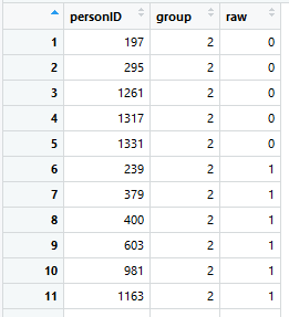
head(elfe)
As you can see, there is no age variable in the data set "elfe", only a person ID, a raw score and a grouping variable. In this case, the grouping variable also serves as a continuous explanatory variable, since children were only examined at the very beginning and in the exact middle of the school year during the test standardization. For example, the value 2.0 means that the children were at the beginning of the second school year, the value 2.5 means that the children were examined in the middle of the second school year. Another possibility would have been to examine children throughout the entire school year. In this case, the duration of schooling would have to be entered as a continuous explanatory variable. To build the grouping variable, the first and second half of each school year could, for exampe, be aggregated into one group respectively.
In the "elfe" data set there are seven groups with 200 cases each, i.e. a total of 1400 cases:
# Display descriptive results
by(elfe$raw, elfe$group, summary)
Ranking: Retrieving Percentiles and Norm Scores
The next step, which is performed automatically when the 'cnorm' function is called, is the ranking of the individual cases per group. Internally, this is done using the rankByGroup function, which determines a rank for each person, returns percentiles, and performs a normal rank transformation that returns T scores (M = 50, SD = 10) by default. In principle, our mathematical method also works without a normal rank transformation, i.e., the procedure could theoretically also be performed with the percentiles. This is useful, for example, if the raw score deviates extremely from the normal distribution or follows a completely different distribution. For most psychological or physical scales, however, the distributions still show enough similarity to the normal distribution even with strong floor and ceiling effects. In these cases, the normal rank transformation usually increases the model fit and facilitates the further computation of the data. In addition to T scores, the normal scores can also be returned as z or IQ scores, or any scale can be defined. Furthermore, it is possible to choose between different ranking methods for handling bindings (RankIt, Blom, van der Warden, Tukey, Levenbach, Filliben, Yu & Huang).
To change the ranking method, the method must be specified with method = x (x = method index; see function help). The norm value can be specified as a T score, IQ score, z score, or using a double vector of M and SD, e.g. scale = c(10, 3) for Wechsler scales. The grouping variable can be disabled by setting group = FALSE. The normal rank transformation is then applied to the entire sample. Please note that there is another function for determining the rank, which works without a discrete grouping variable (rankBySlidingWindow). The rank of each individual subject is then estimated based on the continuous explanatory variable using a sliding window. The width of this window can be specified individually.
However, the sliding window is more of a secondary application and its use is only useful when the age variable is actually continuous. In the 'elfe' data set, on the other hand, the variable 'group' serves both as a continuous explanatory variable and as a discrete grouping variable. We therefore obtain the same norm scores with the 'rankBySlidingWindow' function as with the 'rankByGroup' function in this specific case.
Computing powers and interactions
At this point, where many test developers already stop standardization, the actual modeling process begins. A function is determined which expresses the raw score as a function of the latent person parameter l and the explanatory variable. In the following, we will refer to the latter variable as 'a'. In the 'elfe' example, we use the discrete variable 'group' for a.
To retrieve the mathematical model, all powers of the variables 'l' and 'a' up to a certain exponent k must be computed. Subsequently, all interactions between these powers must also be calculated by simple multiplication. As a rule of thumb, k > 5 leads to over-adjustment. In general, k = 4 or even k = 3 will already be sufficient to model human performance data with adequate precision. Especially the age development can mostly already be covered with the third power. Internally, cNORM uses the computePowers function. It creates new variables in the data object, namely all powers of l (L1, L2, L3, L4 ...), all powers of a (A1, A2, A3, A4 ...) and all products of the powers (L1A1, L1A2, L1A3, ... L4A3, L4A4 ...).
In a single step
cNorm automatically performs all steps and saves the data object under $data, e.g. when modeling the BMI from the CDC dataset:
model.elfe <- cnorm(raw=elfe$raw, group=elfe$group)
head(model.elfe$data)
 |
Installation |
Weighting |
 |